
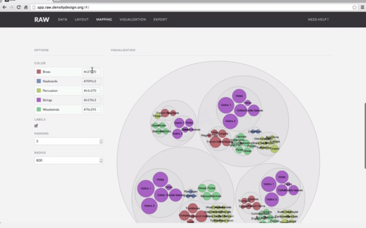
Awesome Tool for Data Visualization
Students walking through the math floor placed a sticker indicating the number of hours of sleep they got the night before. The symmetric and unimodal pattern indicates a normal model with a central tendency of 7 hours and a range of 1 to 18 (?). We can also notice that people tend to round to the nearest hour.

Generalized Linear Model analysis in R
The purpose of this tutorial is to examine a set of data and fit an appropriate model using “glm” to assess the relationship between gender and speeding (fictional data). Controlling for age, we conduct a preliminary investigation as to the effectiveness of the model.
Remember, you can always type “help()” or “example()” at the prompt to get information about R objects.
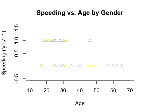
Speeding Data
1. Ungrouped Data
data=read.table(“/Users/—/—/—/speeding.txt”, header=T)
sex=data[,1]-1
#male=1, female=0
age=data[,2]
speeding=data[,3]-1
#was caught speeding in the last year =1, did not get caught speeding in the last year=0
data=cbind(sex,age,speeding)
plot(age,speeding,col=sex+7,pch=sex+1,main=”Speeding vs. Age by Gender”,xlab=”Age”,ylab=”Speeding (‘yes’=1)”,xlim=c(10,70),ylim=c(-.5,1.5))
#fit a GLM using binomial with a logit link function
disp.glm.add=glm(speeding~sex+age,family=binomial(link=logit))
#Check for Extra Binomial Variation—————————-
deviance=disp.glm.add$deviance #select the deviance from the output
df=disp.glm.add$df.residual #select the residual degrees of freedom
deviance/df #=1.122081 not indicative of extra binomial variation (close to 1)
#Examine the Residuals
pearson=summary.lm(disp.glm.add)$residuals
plot(age,pearson,ylim=c(-3,3),ylab=”Pearson Residuals”,xlab=”Age”,main=”Residual Plot”)
abline(h=2)
abline(h=-2)
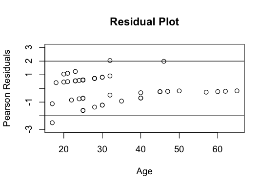
Based on the hypothesis that the model is adequate to describe the relationship, we would expect about 95% of the residuals to fall within the range of -2 and 2. This residual plot reflects this assumption and gives further evidence that the model is appropriate. Further model validation can be obtained using a Hosmer-Lemeshow test for ungrouped/Bernoulli data.
